Inference from Gene Count data: WGDgc

The R package "WGDgc" uses gene count data (number of gene copies) across multiple gene families and multiple species. The background process of gene duplications and gene losses is modelled by a birth and death process. In addition, whole genome duplications (WGD) and whole genome triplications (WGT) are modelled with an instantaneous duplication (or triplication) of all genes present at the time of event, with a probability of retaining the extra gene (or of retaining one of both extra copies for whole genome triplications). The duplication (birth) rate, loss (death) rate and retention rate at each WGD or WGT event are estimated simultaneously using maximum likelihood. A shifted geometric prior distribution is used for the unobserved number of genes at the root. The likelihood can be conditioned on the data collection process. This method is fast. It is further explained here:

Rabier C-E, Ta T., Ane C. : Detecting and locating Whole Genome Duplications on a phylogeny: a probabilistic approach (Molecular Biology and Evolution, 2014, doi:10.1093/molbev/mst263)

R package download

Version 0.9 : R package       Documentation
Version 1.0 : R package       Documentation
Version 1.1 : R package       Documentation
Version 1.2 : R package       Documentation

R package installation

WGDgc depends on the R packages ape, phylobase and phyext.
You can install ape and phylobase from CRAN using the R command install.packages(c("ape","phylobase")) .
The phyext package is no longer on CRAN, but you can install it from source like this:
install.packages("https://cran.r-project.org/src/contrib/Archive/phyext/phyext_0.0.1.tar.gz", repos = NULL, type="source")
Finally, you can install WGDgc also from source, and ask R to do the download for you like this:
install.packages("http://www.stat.wisc.edu/~ane/wgd/WGDgc_1.2.tar.gz", repos = NULL, type="source")

Inference from Sequence data: SPIMAPWGD

This method aims to detect whole genome duplications (WGDs) and to reconstruct the gene trees. It is much slower than the method based on gene count data above (see Rabier et al. 2014), for detecting WGDs. However, it reconstructs the gene tree and SPIMAPWGD can be used to improve gene tree estimation when whole genome duplications have occurred in the group of interest. It is a version of the software SPIMAP of Matthew Rasmussen and Manolis Kellis, which incorporates WGD events. For some background, we refer to the paper "A Bayesian approach for fast and accurate gene tree reconstruction", Rasmussen and Kellis, Mol. Biol. Evol. 28(1):273-290.2011. Some documentation about the SPIMAP package is present here. SPIMAPWGD uses the same arguments as SPIMAP, and also some new arguments. Here, you will find some explanations on how to run SPIMAPWGD. Some examples are given at the end of the page. A version of SPIMAPWGD is available on my github .

SPIMAPWGD is further explained here:
Rabier C-E, Ta T., Ane C. : Detecting and locating Whole Genome Duplications on a phylogeny: a probabilistic approach (Molecular Biology and Evolution, 2014, doi:10.1093/molbev/mst263)

Arguments

input/output

-a,--align : sequence alignments in fasta format

-S,--smap : gene to species map

-s,--stree : species tree in newick format

-p,--param : substitution rate parameters file

-o,--output : prefix for all output filenames

-r,--recon : output reconciliation (optional argument)

Note that SPIMAPWGD will generate the following files : *.tree (final gene tree), *.duplosslastree (total losses, losses at WGD, total duplications, duplications at WGD for final gene tree), *.completeloglikelihood (approximated loglikelihood), and *.topologyprob (topology prior).

sequence model

-k,--kappa : transition/transversion ratio (default estimate)

-f,--bgfreq : base frequencies (A, C, T, G) (default estimate)

dup loss model

-D,--duprate : birth rate

-L,--lossrate : death rate

-LR,--lineagesatroot : parameter of the prior geometric distribution for the number of lineages at the root. Inverse of the average number of lineages at the root. (default 0.95, i.e. an average of 1.053 lineages at the root)

-OB,--observingsomething : 1 for conditioning on observing something, 2 for at least one gene on each side of the root (default 1)

search options

-i,--niter : number of iterations (default 100)

-g,--proposal-gene-topology : 0 for NNI, 1 for SPR, 2 for SubtreeSlide (default 2)

help informations

-V,--verbose : 0 for quiet, 1 for low, 2 for medium, 3 for high

--log : specify a file name for saving log information

-h, --help : display help information

--informationduploss : output total losses, losses at WGD, total duplications, duplications at WGD (corresponding to some sampled trees)

--treesampled : output sampled trees (warning : does not give the full list)

How to include a WGD in the species tree

SPIMAPWGD requires a species tree in the Newick format. In order to include a Whole Genome Duplication in the species tree, just add a supplementary node called "WGDp" where p is the value of the probability of loss at the WGD.

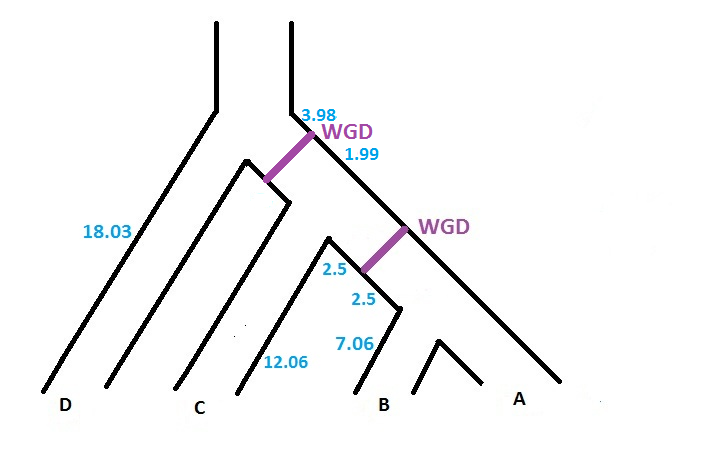
For instance, if we consider a species tree with 4 taxon (A,B,C,D), and if we want to specify that a WGD, with probability of loss 0.10, is present just at the middle of the branch located before the speciation A|B, the input file corresponding to the figure below will be

((( (A:7.06, B:7.06 ):2.50)WGD0.10:2.50, C:12.06 ):5.97, D:18.03 ) ;

The software can handle several WGDs with different probability of loss. However, each WGD has to be located on a different branch of the species tree. So, if we want to add another WGD (with probability of loss 0.12) on the branch located just above the previous WGD (cf. figure below), the input file will be

(((((A:7.06,B:7.06):2.50)WGD0.10:2.50,C:12.06):1.99)WGD0.12:3.98,D:18.03);

How to handle substitution rates

We just have to use the same input file as in SPIMAP. In other words, we do not have to take into account that some WGD are present inside the species tree

About the reconciliation

As in the original version of SPIMAP, the software gives the reconciliation (with the option -r). It now specifies which nodes are reconciled at the WGD. Note that when several WGDs are located in the species tree, before interpreting the reconciliation file (.recon), we have to know the code associated to each WGD. This code is given on the screen when we run SPIMAPWGD. In particular, SPIMAPWGD describes the 2 WGDs of the figure above in the following way :

WGD event number0:
child node : n5
loss probability: 0.100000
percent distance: 0.500000
total distance: 5.000000
distance 'before': 2.500000
distance 'after': 2.500000

WGD event number1:
child node : n4
loss probability: 0.120000
percent distance: 0.666667
total distance: 5.970000
distance 'before': 3.980000
distance 'after': 1.990000

'Total distance' gives the length of the branch on which the WGD is placed.
'Percent distance' indicates where the WGD is located on the branch, as a percentage of the total distance starting from the parent node.
Distances 'before'/'after' are the distances before/after the WGD.

We can see that the oldest WGD has the number 1, whereas the most recent has the number 0.

Recall that the reconciliation file (.recon) has 3 columns. The first column refers to the gene tree whereas the second column refers to the species tree. On each row, a node of the gene tree (first column) is reconciled to a node of the species tree (second column). The third column indicates the corresponding evolutionary event : 'gene', 'speciation', 'dup' (for duplication), 'WGD'. Note that when the evolutionary event is a WGD, column 2 also gives the number associated the WGD.

Example on reconciliation using our species tree with only one WGD

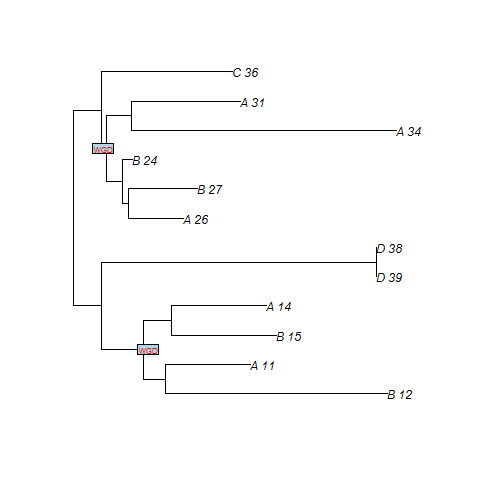
We give here an example of gene tree (simulated from our species tree with only one WGD) obtained by SPIMAPWGD, and also some rows of the reconciliation file (.recon) :

A_11	A	gene
B_12	B	gene
B_15	B	gene
C_36	C	gene
n4	n5	spec
n6	D	dup
n8	WGD_at0	WGD
n3	WGD_at0	WGD
...	...	...

SPIMAPWGD finds two duplications at the WGD. n8 and n3 are the nodes of the gene tree that map at the WGD (cf. figure). Note that file .duplosslasttree gives the total number of losses, the number of losses at the WGD, the total number of duplications and the number of duplications at the WGD.

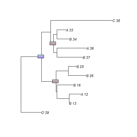
Example of reconciliation using our species tree with two WGDs

A_10	A	gene
B_11	B	gene
C_12	C	gene
n3	WGD_at0	WGD
n2	WGD_at1	WGD
n8	WGD_at0	WGD
...	...	...

SPIMAPWGD finds three duplications at the WGDs. n2 is the node of the gene tree which maps to the WGD number 1. n3 and n8 are the nodes which maps to the WGD number 0. We recall that WGD number 1 is the oldest WGD whereas WGD number 0 is the most recent.

Examples on how to run SPIMAPWGD

For more details, download TUTORIAL.tar.gz and open the file README.sh. You will find the same examples as the ones present on this page. In the folder "dnawith1WGD" (resp. "dnawith2WGD"), you will find 20 data sets, generated with the species tree with one WGD (resp. two WGDs).

Some results using a data set of 16 fungal species

As explained in the paper, we ran SPIMAPWGD on a data set of 16 fungal species. We considered the same gene clusters as in Butler et al. (Nature 2009), that is to say 9209 gene families, downloaded from http://compbio.mit.edu/candida . The fungal species tree comes also from this recent study. The WGD was placed at the middle of the branch (arbitrarily) of the species tree where a putative WGD happened in yeast. An example of species tree with probability of loss 0.4 can be downloaded here. You will also find a table which summarizes our results, and the gene trees found for each family (gene family sizes: 3 to 40, 41 to 56, 57 to 130 , readme.txt).